Important note 1: To be able to run all the examples below, please ensure that you have built your LAMMPS library with the following packages: EXTRA-DUMP, MOLECULE, RIGID, and QEQ. See installation and the relevant LAMMPS documentation page for more information.
Important note 2: The Adsorption/Desorption and Phosphates examples produce trajectory files (i.e., xyz) with varying (from timestep to timestep) numbers of atoms. VMD cannot handle such trajectory files and will only draw the initial state (i.e., the substrate). Consider using another visualization software (e.g., OVITO) capable of handling varying atoms.
Your first PAPRECA simulation: Brownian Diffusion (random walk)
The Brownian motion example can be found in the ./Examples/Brownian Self Diffusion/ folder.
Even though PAPRECA is an extension for LAMMPS, it can be deployed to perform pure off-lattice kMC studies. In this example, we will demonstrate how PAPRECA can be used to calculate the temporal evolution of the spatial distribution of Brownian particles confined in a box [1], [2].
LAMMPS and PAPRECA input files
As far as the LAMMPS input file (i.e., in_kmc.lmp) is concerned, note that:
- The create_atoms command is deployed to create a cluster of atoms of type 1 in the middle of the simulation box.
- This simulation is a pure kMC simulation. The choice of pair_style does not make any difference at all.
- The pair_coeff 1 1 for the "lj/cut" potential is defined to set the sigma value (i.e., 2.84642 Angstroms). Such value is used to perform collision searches for the diffusion event (see create_DiffusionHop command, sigmas_options command, and init_sigma command).
For more information regarding the used LAMMPS commands consider visiting the relevant documentation pages.
When it comes to the PAPRECA input file (i.e., in_kmc.ppc), note that:
- An MD stage is performed every 10 kMC stages. The MD stage produces a trajectory file without affecting the system dynamics.
- A diffusion template is set (see create_DiffusionHop command) and random_diffvecs with the "3D" option were activated to allow atoms to diffuse anywhere in the 3D space (random_diffvecs command).
Execution
The easiest way to run PAPRECA is by running one of the following commands in the directory where the input files are located:
or
or
or
Important note 1: Redirecting the screen output to an external file (e.g., log.hybrid) is generally not advised. Such external files can occupy a considerable amount of disc space and potentially lower the performance of PAPRECA. LAMMPS' screen output is already redirected to the log.lammps file and some information from PAPRECA is written on the papreca.log file.
Important note 2: It is better advised to run the Brownian example as an automated test (see below).
To run the Brownian motion example as an automated test use "test_brownian.sh" bash script in the example folder directory. Note that, you might have to modify the "papreca_dir" variable in your "test_brownian.sh" script so it points to the path of your PAPRECA executable. If you wish to use "python" instead of "python3" you will also have to modify "test_brownian.sh". In any case, the Brownian test can be executed through one of the following commands:
or
The automated test runs PAPRECA with the relevant LAMMPS and PAPRECA input files. After the simulation finishes, it calls a python script to plot the spatial distributions of atoms (as exported in the distribution files in the results folder) at various times. The python script also exports an image file in the parent directory named distributions.png.
Results
The obtained spatial distribution of diffused atoms can be found below:
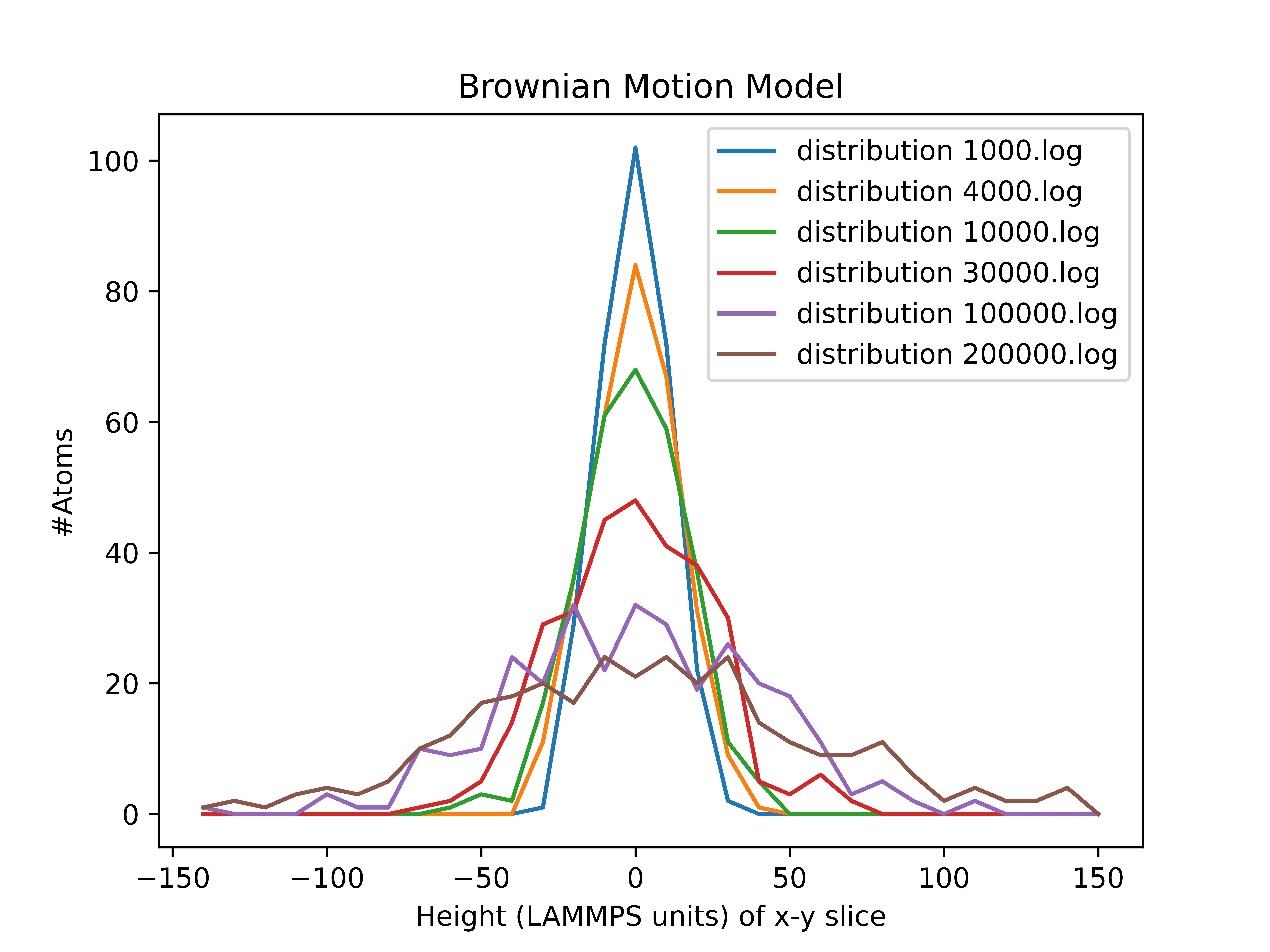
Where it can be observed that the distribution can be described by a bell-shaped curve. As expected, the standard deviation (STD) of the distribution becomes greater over time [1], [2], [3].
Bibliography
[1] wikipedia
[3] Lavenda, B. H. "Nonequilibrium Statistical Thermodynamics.", Dover Publications, 2019
Monoatomic adsorption and desorption
The Monoatomic adsorption and desorption example can be found in the ./Examples/Simple Adsorption/ folder.
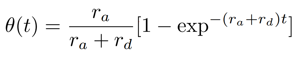
Once again, this is a pure kMC example (see another pure kMC example here: Your first PAPRECA simulation: Brownian Diffusion (random walk)). The system comprises an FFC substrate of atoms of type 1. Atoms of type 2 can adsorb, or desorb on the surface with a given probability. The adsorption sites are directly above the parent atoms, at a distance of depo_offset (see create_Deposition command). The ultimate goal of this test is to accurately capture the surface coverage as a function of time. The analytic solution for the surface coverage is [1], [2]:
LAMMPS and PAPRECA input files
For the PAPRECA and LAMMPS input files note that:
- This is a pure off-lattice kMC example. Hence, a MD (LAMMPS) stage is invoked every 250 kMC stages (as set in the PAPRECA input file) to produce trajectory files and does not affect the dynamics of the system. See the relevant section in the Brownian motion example (i.e., LAMMPS and PAPRECA input files) for additional information.
- The pair_coeff command was used (in the LAMMPS input file) to set the sigma values of the pairs of atoms (see create_DiffusionHop command, sigmas_options command, and init_sigma command).
- Two predefined events are defined (in the PAPRECA input file) for this simulation: a deposition event (see create_Deposition command) and a monoatomic desorption event (see create_MonoatomicDesorption command).
- random_depovecs (in the PAPRECA input file) were set to "no" so that adsorption sites can be directly above the parent atoms.
Note: See export_SurfaceCoverage command for additional information regarding the calculation of surface coverage.
Execution
This example is meant to be executed as a batch test. To run the batch test, modify the "papreca_dir" directory of your "test_simple_adsdep.sh" file so it points to the path of your PAPRECA executable. If you wish to use "python" instead of "python3" you will also have to modify "test_simple_adsdep.sh". The automated test can be executed through one of the following command:
or
The batch script will access and modify the template PAPRECA and LAMMPS input files (located in the ./template folder), and perform a series of PAPRECA simulations for different combinations of adsorption/desorption rates. After performing each run, the batch script will call a python script that plots the surface coverage solution as calculated by PAPRECA alongside the analytic solution and exports an image file (in the ./results folder).
Results
Below you can find a gif of the the system trajectory (after it reaches equilibrium) as well as the relevant surface coverage plot corresponding to an adsorption/desorption rate ratio of 5:
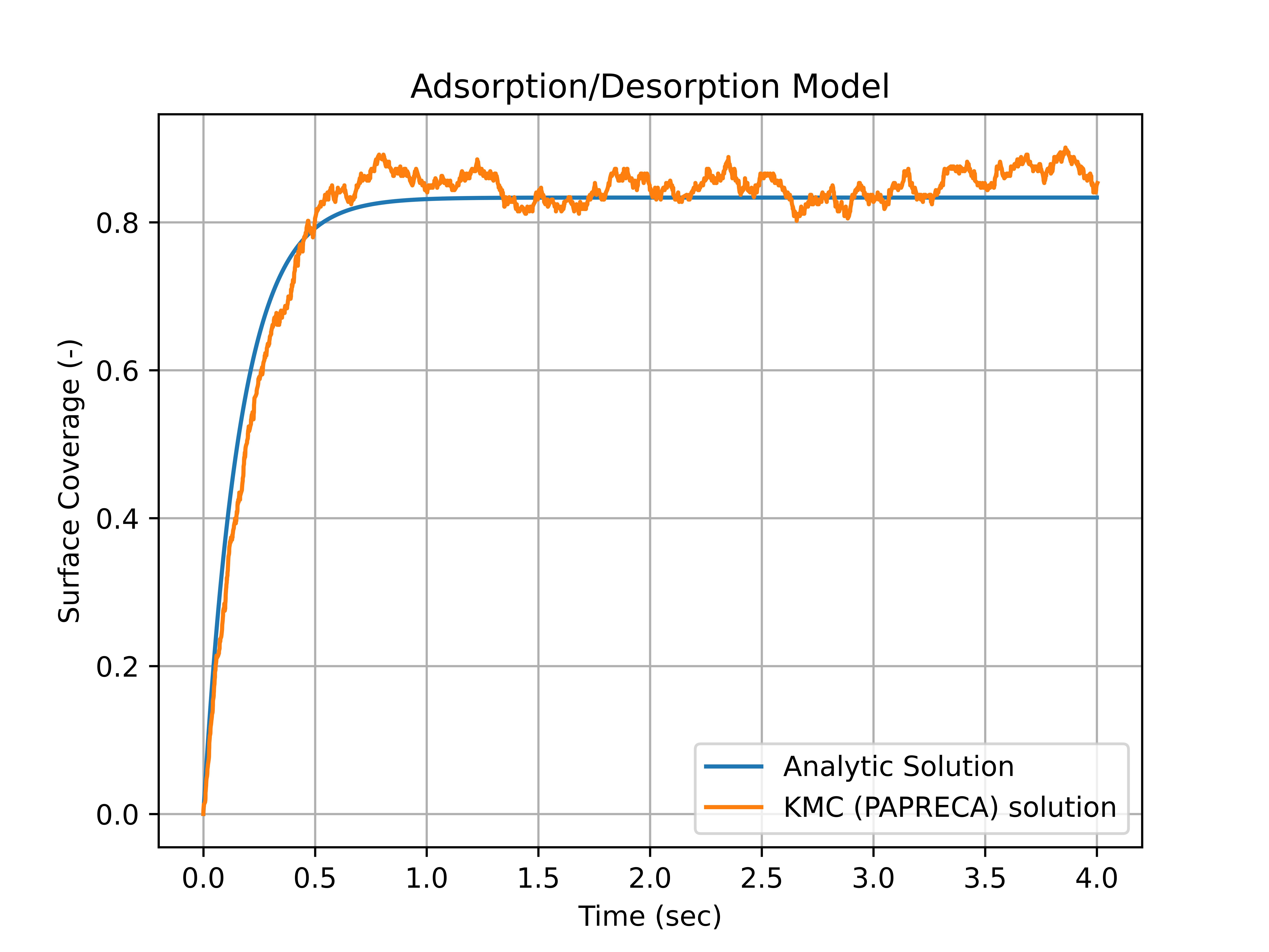
Where it can be concluded that the PAPRECA solution matches the analytic solution closely. Of course, a good agreement between the PAPRECA and analytic solutions is observed for all other tested adsorption/desorption rate ratios (see ./results folder).
Bibliography
[1] Fichthorn, K.A. and Weinberg, W.H. "Theoretical foundations of dynamic Monte Carlo simulations." Journal of Chemical Physics, vol. 95, 1991
[2] KMC course from the University of Illinois.
Film growth from the thermal decomposition of tricresyl phosphate (TCP) molecules on a Fe110 surface.
DISCLAIMER: This example requires considerably more time to finish than the Your first PAPRECA simulation: Brownian Diffusion (random walk) and Monoatomic adsorption and desorption simulations. See here for more information regarding the scalability of this example and the required runtime. Also, consider reducing the total number of kMC steps of kMC_steps for shorter runs.
The files associated with this example can be found in the ./Examples/Phosphate Film Growth from TCP on Fe110/
This example demonstrates the full capabilities of the software. The example is hybrid (i.e., MD/kMC) and involves bond-formation (see create_BondForm command), bond-breaking (see create_BondBreak command), deposition (see create_Deposition command), and diffusion (see create_DiffusionHop command) events. Following the execution of each predefined event, the LAMMPS library is called (i.e., an MD stage is performed) to relax the interatomic forces and thermalize the system to the target temperature. For a detailed discussion regarding the results from our off-lattice hybrid kMC/MD runs on thin films from TCP molecules consider reading our paper on Computational Materials Science [1]. A hybrid kMC/MD code (written in FORTRAN), specifically designed to study the decomposition of TCP molecules on Fe(110), was used for all simulations in this paper. Nonetheless, the film-growth model can be reproduced in PAPRECA by using the PAPRECA and LAMMPS inputs files, as well as the param.qeq (declaring the coefficients of the QeQ charge equilibration scheme) and TCP.in (initializing an mmm-TCP molecule) files located in the example folder. Note that, the following changes/improvements were made to the old phosphates model [1]:
- In the newest model, Carbon and Hydrogen species are not deleted from the system following C-O bond breaks.
- The reflective walls on the x-y plane above the growing film were removed. Instead, the latest model periodically removes atoms located 20 Angstroms above the film (using the desorption command in the PAPRECA input file).
LAMMPS and PAPRECA input files
The PAPRECA and LAMMPS input files required to run this example are located in the parent example directory. Comments have been added in both input files to explain the purpose of specific commands.
Execution
To run this example, you should execute the following command:
or
or
Results
A complete discussion regarding the results of this study is provided in our previous paper (Ntioudis et al. [1]). Below we showcase the capabilities of the software by providing two example curves that can be produced by PAPRECA:
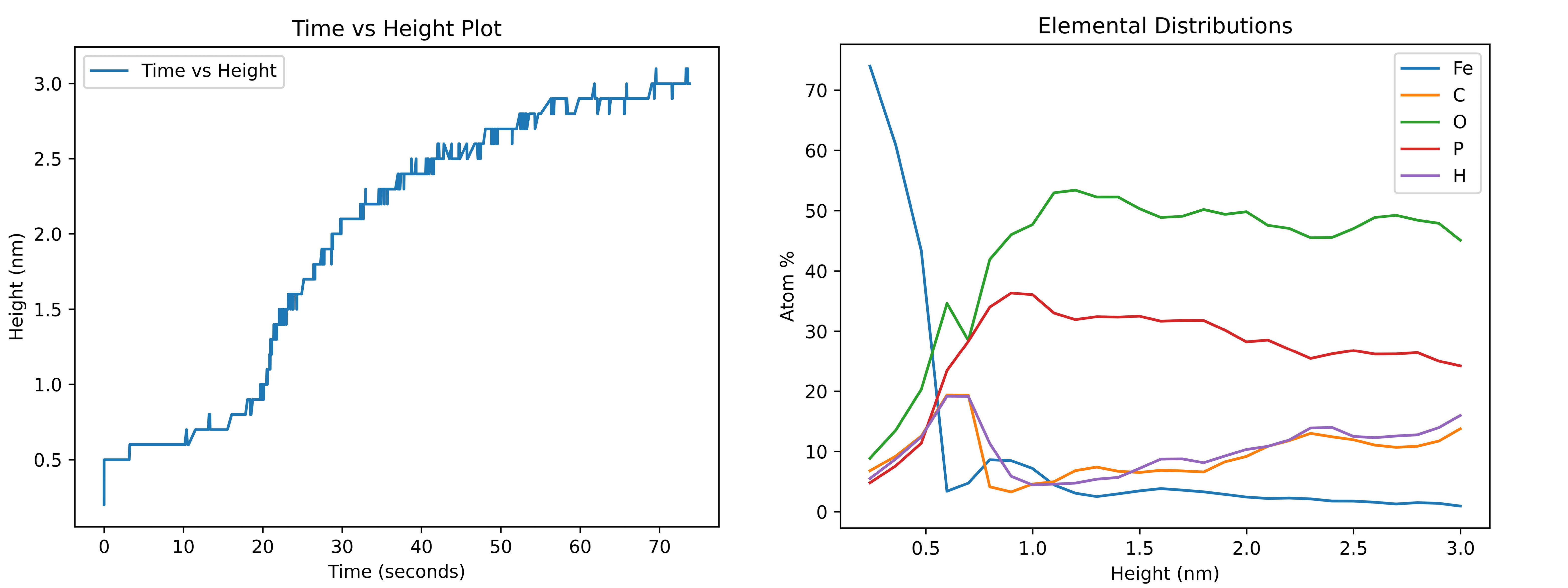
Where the curve on the left is a height-time plot generated by export_HeightVtime command and the elemental distribution lines on the right can be exported through the export_ElementalDistributions command. Note that, both graphs have been generated using the respective export files at the end of the run (i.e., heightVtime.log after 12000 PAPRECA steps and distributions 12000.log). Furthermore, to reduce noise in the elemental distributions graph running averages of atomic percentages were calculated for every five consecutive height bins.
Bibliography
[1] Ntioudis, S., et al. "A hybrid off-lattice kinetic Monte Carlo/molecular dynamics method for amorphous thin film growth." Computational Materials Science, vol. 229, 2023
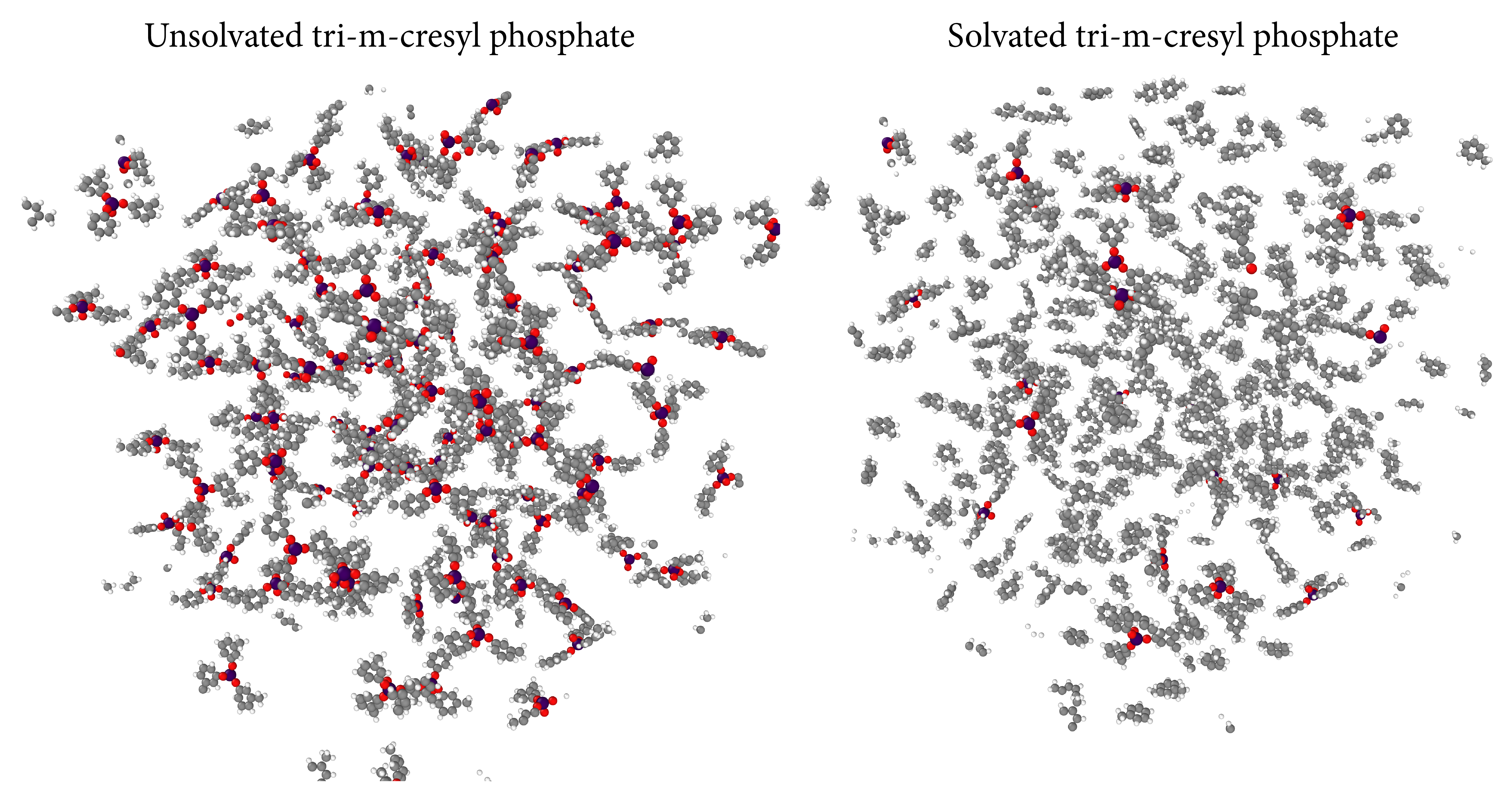
Organic solvents
The TCP and Toluene subdirectory in the Examples folder contains the input files for 1) a system comprising solely tri-m-cresyl phosphate (mmm-TCP) molecules, and 2) a system of mmm-TCP molecules in a toluene solvent. Both examples are hybrid kMC/MD runs and include a set of (dummy) bond-formation and bond-breaking events. These examples showcase the capabilities of PAPRECA when it comes to capturing solvent/solute interactions. Furthermore, the examples allow for performance comparisons between solvated and unsolvated systems.
Execution
Similarly to the previous sections, the examples can be initiated by calling the PAPRECA executable with either the mpiexec or the mpirun command:
or